Joins Tutorial

Introduction to joining datasets using dplyr

This document has been adapted and extended by Michael Hallquist and Benjamin Johnson from Jenny Bryan’s dplyr joins tutorial (http://stat545.com/bit001_dplyr-cheatsheet.html). Animations were developed by Garrick Aden-Buie. The goal is to develop an intuition of the four major types of two-table join operations: inner, left, right, and full. We’ll also get into using joins to identify areas of match or mismatch between two datasets (using semi- and anti-joins).

Warning: The `file` argument of `read_csv()` should use `I()` for literal data as of
readr 2.2.0.
  
  # Bad (for example):
  read_csv("x,y\n1,2")
  
  # Good:
  read_csv(I("x,y\n1,2"))

Superheroes table

name	alignment	gender	publisher
Magneto	bad	male	Marvel
Storm	good	female	Marvel
Mystique	bad	female	Marvel
Batman	good	male	DC
Joker	bad	male	DC
Catwoman	bad	female	DC
Hellboy	good	male	Dark Horse Comics

Publishers Table

publisher	yr_founded
DC	1934
Marvel	1939
Image	1992

Mutating joins: inner, left, right, full

“Mutating” joins combine variables from two datasets on the basis of one or more keys that match between datasets. In the case of these datasets, notice they share the “publisher” column.

N.B.: By default, dplyr will search for common columns across datasets as the matching keys (natural join). If you want to control the process, specify the key using by.

inner join

Require match in both datasets (non-matching rows are dropped)

For those of you who are visual learners, conceptually, imagine the following two simple datasets:

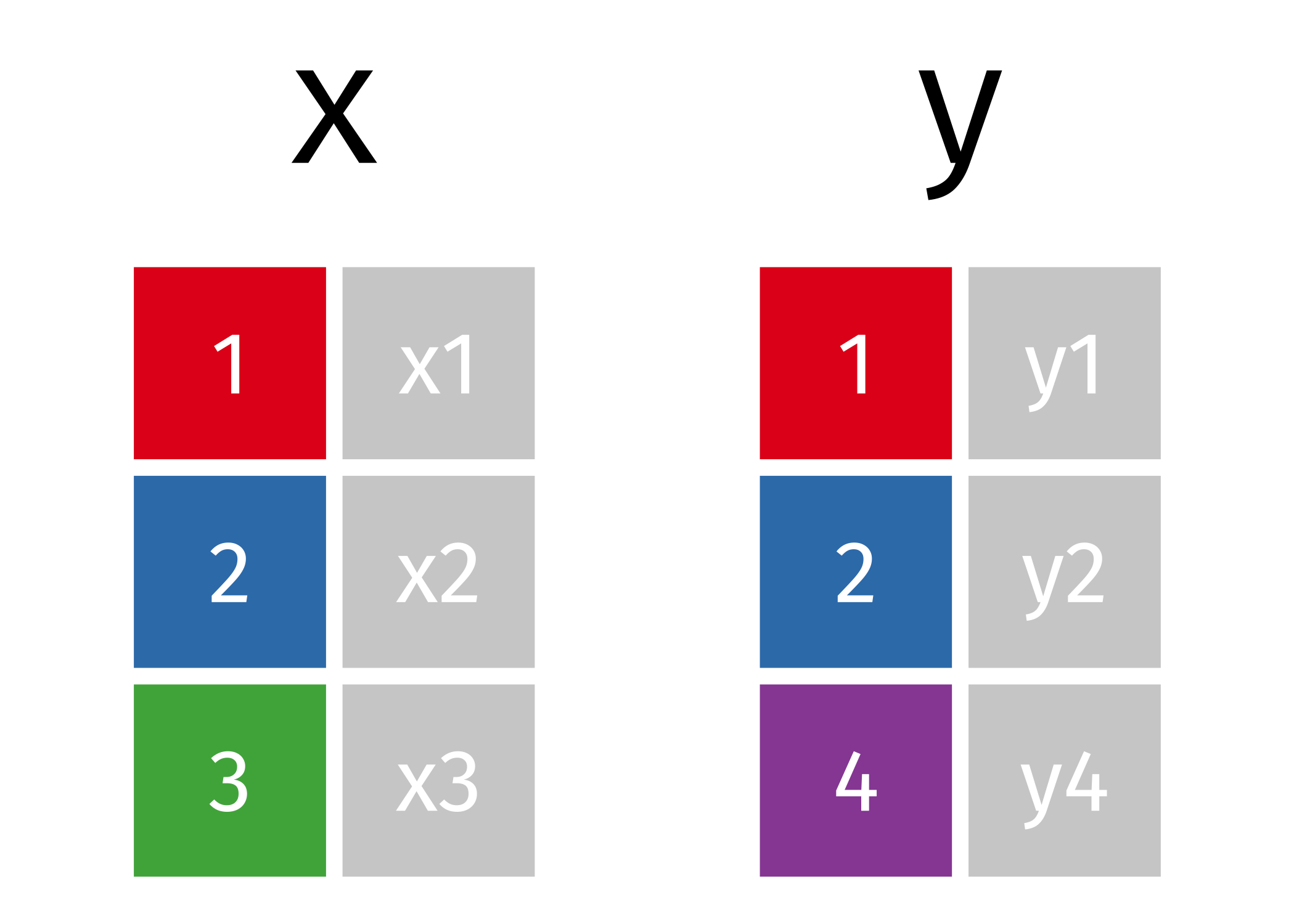
An inner join combines the two datasets and drops the non-matching rows like so:

Let’s try it with our superhero data.

#*NB*: Here, we retain the joined dataset as ijsp
ijsp <- inner_join(x=superheroes, y=publishers)
print(ijsp)

# A tibble: 6 × 5
  name     alignment gender publisher yr_founded
  <chr>    <chr>     <chr>  <chr>          <dbl>
1 Magneto  bad       male   Marvel          1939
2 Storm    good      female Marvel          1939
3 Mystique bad       female Marvel          1939
4 Batman   good      male   DC              1934
5 Joker    bad       male   DC              1934
6 Catwoman bad       female DC              1934

Same idea, just explicit declaration of key (i.e., “publisher”)

#note that we've cut the x=, y= as this optional
inner_join(superheroes, publishers, by="publisher")

name	alignment	gender	publisher	yr_founded
Magneto	bad	male	Marvel	1939
Storm	good	female	Marvel	1939
Mystique	bad	female	Marvel	1939
Batman	good	male	DC	1934
Joker	bad	male	DC	1934
Catwoman	bad	female	DC	1934

Notice both Hellboy (from the superheroes dataset) and Image comics (from the publishers dataset) were dropped.

left join

Keep all rows in left-hand ‘x’ dataset (i.e., superheroes). Add columns from publishers where there is a match. Fill in NA for non-matching observations.

left_join(superheroes, publishers, by="publisher")

name	alignment	gender	publisher	yr_founded
Magneto	bad	male	Marvel	1939
Storm	good	female	Marvel	1939
Mystique	bad	female	Marvel	1939
Batman	good	male	DC	1934
Joker	bad	male	DC	1934
Catwoman	bad	female	DC	1934
Hellboy	good	male	Dark Horse Comics	NA

right join

Keep all rows in right-hand ‘y’ dataset (i.e., publishers). Add columns from superheroes where there is a match. Fill in NA for non-matching observations.

# Note the shift to using dplyr piping
# This achieves the same purpose, but may be preferred by those who love pipes
superheroes %>% right_join(publishers, by="publisher")

name	alignment	gender	publisher	yr_founded
Magneto	bad	male	Marvel	1939
Storm	good	female	Marvel	1939
Mystique	bad	female	Marvel	1939
Batman	good	male	DC	1934
Joker	bad	male	DC	1934
Catwoman	bad	female	DC	1934
NA	NA	NA	Image	1992

full join

Keep all rows in left-hand ‘x’ (superheroes) and right-hand ‘y’ (publishers) datasets.

Resulting dataset will have all columns of both datasets, but filling in NA for any non-matches on either side (denoted as blank spaces below).

superheroes %>% full_join(publishers, by="publisher")

name	alignment	gender	publisher	yr_founded
Magneto	bad	male	Marvel	1939
Storm	good	female	Marvel	1939
Mystique	bad	female	Marvel	1939
Batman	good	male	DC	1934
Joker	bad	male	DC	1934
Catwoman	bad	female	DC	1934
Hellboy	good	male	Dark Horse Comics	NA
NA	NA	NA	Image	1992

One-to-many join

Note that when there are non-unique matches, the join adds all possible combinations.

This occurs in a one-to-many join, where a single observation in table A relates to multiple observations in table B. For this scenario, the single table A observation will be replicated onto multiple rows to match the multiple observations in table B.

Let’s say you wanted to examine how mood ratings provided over many days relate to demographic characteristics such as age.

person	day	mood
Jeff	1	3
Jeff	2	3
Jeff	3	10
Jeff	4	2
Jeff	5	6
Jeff	6	5

person	bio_sex	age	height_in
Jeff	Male	15	66
Ping	Male	18	71
Karla	Female	19	60

person	bio_sex	age	height_in	day	mood
Jeff	Male	15	66	1	3
Jeff	Male	15	66	2	3
Jeff	Male	15	66	3	10
Jeff	Male	15	66	4	2
Jeff	Male	15	66	5	6
Jeff	Male	15	66	6	5
Ping	Male	18	71	1	4
Ping	Male	18	71	2	6
Ping	Male	18	71	3	9
Ping	Male	18	71	4	10
Ping	Male	18	71	5	5
Ping	Male	18	71	6	3
Karla	Female	19	60	1	9
Karla	Female	19	60	2	9
Karla	Female	19	60	3	9
Karla	Female	19	60	4	3
Karla	Female	19	60	5	8
Karla	Female	19	60	6	10

Notice how the demographic variables are replicated on rows for each day of mood ratings. If both tables have duplicates for the key, joins can produce many-to-many combinations and a large increase in rows.

Filtering joins: semi_join and anti_join

Filtering joins use specific criteria to identify observations (rows) from one table that exist or don’t exist in another table.

These joins are typically used for diagnosing mismatch between two overlapping datasets. That is, filtering joins are most useful for data quality assurance checks.

semi_join

retain observations (rows) in x that match in y

Observations in superheroes that match in publishers

Notice that this is different from the left_join shown above as the data from y is not kept. That is the fundamental difference between ‘mutating joins’ (e.g., left_join) and ‘filtering joins’ (e.g., semi_join).

semi_join(superheroes, publishers, by="publisher")

name	alignment	gender	publisher
Magneto	bad	male	Marvel
Storm	good	female	Marvel
Mystique	bad	female	Marvel
Batman	good	male	DC
Joker	bad	male	DC
Catwoman	bad	female	DC

Observations in publishers that match in superheroes

semi_join(publishers, superheroes, by="publisher")

publisher	yr_founded
DC	1934
Marvel	1939

This can be useful if you have a dataset of your data of interest and another dataset that indicates which of your participants/observations you want to remove or filter out.

anti_join

observations in x that are not matched in y Note that this is similar to setdiff in base R

Observations in superheroes that don’t match in publishers

anti_join(superheroes, publishers, by="publisher")

name	alignment	gender	publisher
Hellboy	good	male	Dark Horse Comics

Observations in publishers that don’t match in superheroes

publishers %>% anti_join(superheroes, by="publisher")

publisher	yr_founded
Image	1992

This can be useful if you are trying to identify extra participants/observations that may have snuck into one dataset (x) or been deleted in another (y).

Joining multiple datasets

Joining can be done repeatedly across multiple datasets. The following code, for instance, joins datasets two at a time from left to right in the list. The result of a two-table join becomes the ‘x’ dataset for the next join of a new dataset ‘y’.

set.seed(123)
df1 <- data.frame(id=1:10, x=rnorm(10), y=runif(10))
df2 <- data.frame(id=1:11, z=rnorm(11), a=runif(11))
df3 <- data.frame(id=2:10, b=rnorm(9), c=runif(9))

print(df1)

   id           x         y
1   1 -0.56047565 0.8895393
2   2 -0.23017749 0.6928034
3   3  1.55870831 0.6405068
4   4  0.07050839 0.9942698
5   5  0.12928774 0.6557058
6   6  1.71506499 0.7085305
7   7  0.46091621 0.5440660
8   8 -1.26506123 0.5941420
9   9 -0.68685285 0.2891597
10 10 -0.44566197 0.1471136

print(df2)

   id          z          a
1   1  1.7869131 0.79892485
2   2  0.4978505 0.12189926
3   3 -1.9666172 0.56094798
4   4  0.7013559 0.20653139
5   5 -0.4727914 0.12753165
6   6 -1.0678237 0.75330786
7   7 -0.2179749 0.89504536
8   8 -1.0260044 0.37446278
9   9 -0.7288912 0.66511519
10 10 -0.6250393 0.09484066
11 11 -1.6866933 0.38396964

print(df3)

  id          b         c
1  2 -0.5996083 0.6680556
2  3 -0.1294107 0.4176468
3  4  0.8867361 0.7881958
4  5 -0.1513960 0.1028646
5  6  0.3297912 0.4348927
6  7 -3.2273228 0.9849570
7  8 -0.7717918 0.8930511
8  9  0.2865486 0.8864691
9 10 -1.2205120 0.1750527

dftemp <- full_join(df1, df2, by="id")
dffinal <- full_join(dftemp, df3, by="id")

#alternative way to combine that avoids temporary variables
Reduce(function(x, y) full_join(x, y, by="id"), list(df1, df2, df3))

id	x	y	z	a	b	c
1	-0.5604756	0.8895393	1.7869131	0.7989248	NA	NA
2	-0.2301775	0.6928034	0.4978505	0.1218993	-0.5996083	0.6680556
3	1.5587083	0.6405068	-1.9666172	0.5609480	-0.1294107	0.4176468
4	0.0705084	0.9942698	0.7013559	0.2065314	0.8867361	0.7881958
5	0.1292877	0.6557058	-0.4727914	0.1275317	-0.1513960	0.1028646
6	1.7150650	0.7085305	-1.0678237	0.7533079	0.3297912	0.4348927
7	0.4609162	0.5440660	-0.2179749	0.8950454	-3.2273228	0.9849570
8	-1.2650612	0.5941420	-1.0260044	0.3744628	-0.7717918	0.8930511
9	-0.6868529	0.2891597	-0.7288912	0.6651152	0.2865486	0.8864691
10	-0.4456620	0.1471136	-0.6250393	0.0948407	-1.2205120	0.1750527
11	NA	NA	-1.6866933	0.3839696	NA	NA

Alternative using pipeline (less extensible)

mergedf <- df1 %>% full_join(df2, by="id") %>% full_join(df3, by="id")