Working with annotations and labels in ggbrain
Michael Hallquist
26 Oct 2022
Source:vignettes/ggbrain_labels.Rmd
ggbrain_labels.RmdCategorical images in ggbrain
Many visualizations of brain data rely on continuous-valued images containing intensities or statistics. For example, we might wish to visualize the z-statistics of a general linear model. These are classic “statistical parametric maps.”
Yet, many images contain integers whose values represent a priori regions of interest or clusters identified using familywise error correction methods. Brain atlases are a common example of integer-valued images. Here, we demonstrate the visualization of a cortical parcellation developed by Schaefer and colleagues (2018).
Schaefer, A., Kong, R., Gordon, E. M., Laumann, T. O., Zuo, X.-N., Holmes, A. J., Eickhoff, S. B., & Yeo, B. T. T. (2018). Local-global parcellation of the human cerebral cortex from intrinsic functional connectivity MRI. Cerebral Cortex, 28, 3095-3114.
This version of the atlas contains 200 cortical parcels (in the paper, they show 100-1000 parcels).
## [1] 201At a basic level, we can visualize this image in the same way as continuous images, as described in the ggbrain introduction document.
gg_obj <- ggbrain() +
  images(c(underlay = underlay_file, atlas = schaefer200_atlas_file)) +
  slices(c("z = 30", "z=40")) +
  geom_brain(definition = "underlay", show_legend = TRUE, name="Anatomical") +
  geom_brain(definition = "atlas", name = "Parcel number")

plot(gg_obj)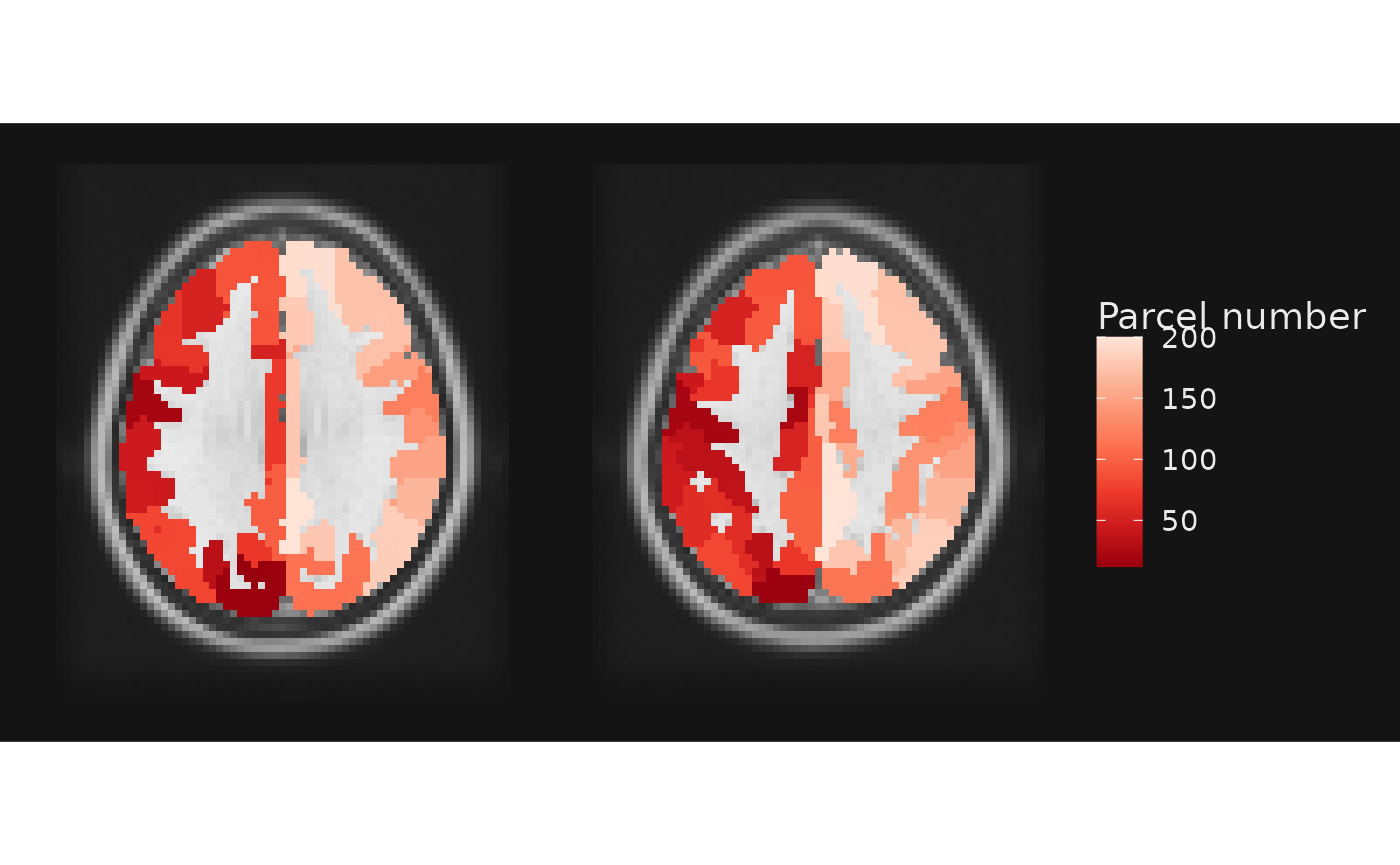
As we can see, however, the continuous values represent discrete
parcels in the atlas. Thus, we may wish to use a categorical/discrete
color scale to visualize things. As with base ggplot2, we
can wrap the fill column in factor to force conversion to a
discrete data type.
Note that the numeric value of any image in a ggbrain
object is always called value. And thus, for
geom_brain and geom_outline objects, the
default aesthetic mapping is aes(fill=value).
gg_obj <- ggbrain() +
  images(c(underlay = underlay_file, atlas = schaefer200_atlas_file)) +
  slices(c("z = 30", "z=40")) +
  geom_brain(definition = "underlay") +
  geom_brain(definition = "atlas", name = "Parcel number",
             mapping = aes(fill = factor(value)), fill_scale = scale_fill_hue())

plot(gg_obj)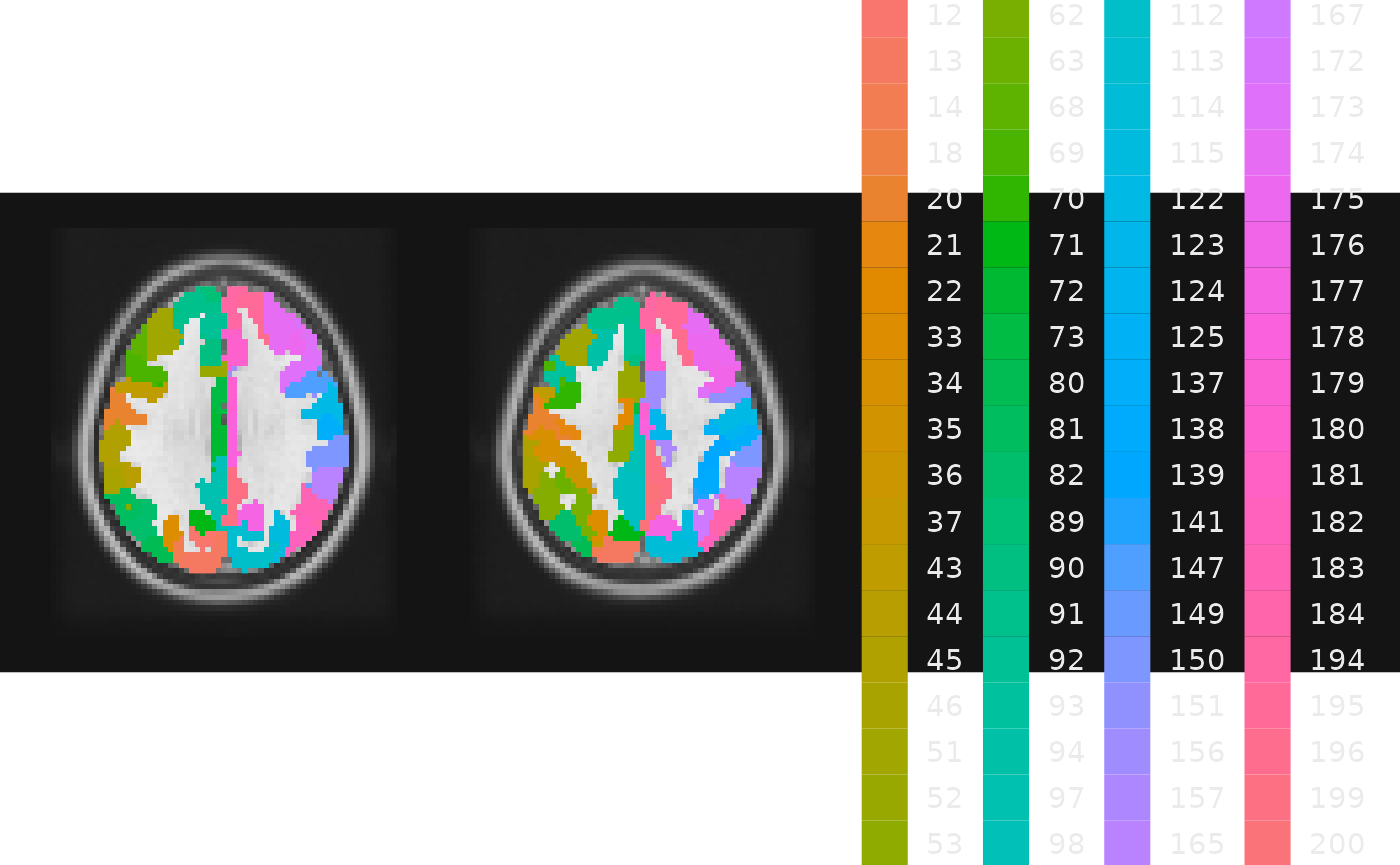
This is a lot to take in! It’s not especially easy to resolve 70+ parcels by their color…
We could use use subsetting syntax in the layer definition to reduce the number of parcels. For example, perhaps we’re interested in just the first 20.
gg_obj <- ggbrain() +
  images(c(underlay = underlay_file, atlas = schaefer200_atlas_file)) +
  slices(c("z = 30", "z=40")) +
  geom_brain(definition = "underlay") +
  geom_brain(definition = "atlas[atlas < 20]", name = "Parcel number",
             mapping = aes(fill = factor(value)), fill_scale = scale_fill_hue()) +
  render()

plot(gg_obj)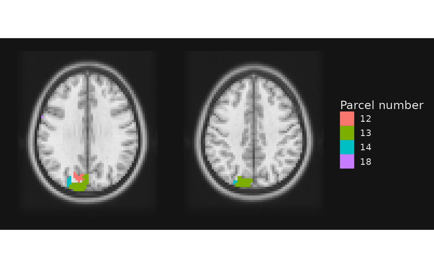
This is more manageable, though uninspiring.
Mapping image values to labels
Categorical images typically contain one integer value at each voxel. The values could be the cluster number from a clusterization procedure (e.g., AFNI’s 3dClusterize), a region of interest from a meta-analytically derived mask (e.g., NeuroSynth), or an atlas value from a stereotaxic atlas (e.g., the Schaefer atlas used here).
Regardless, the conceptual view is that each integer in the image represents a category of interest. Moreover, we may wish to label these categories with more descriptive labels, not simply the integer value. Thus, integers in an image give us the locations of regions to be labeled, while a separate data table provides the integers <-> labels mapping.
Our labels could be region names, intrinsic networks, or other
features we wish to highlight on the display. Regardless, there are two
major ways in which labels can be displayed on a ggbrain
plot: mapping the labels to colors displayed in the legend or adding
text annotations at the locations of the regions. We will review these
two approaches in turn.
First, however, let’s see how we tell ggbrain to merge
labels with an integer-valued NIfTI image. Above, we read in a CSV file
containing labels for regions in the Schaefer 200 parcellation. These
were generated in part using AFNI’s whereami command with the centroids
of each region serving as an input. This gives us automated labels that
we may wish to display on the plot. The CSV also contains a columns
called network that refers to the network mapping to the
Yeo 2011 7-network parcellation.
| roi_num | hemi | x | y | z | network | MNI_Glasser_HCP_v1.0 | Brainnetome_1.0 | CA_ML_18_MNI | schaefer_region | custom_label |
|---|---|---|---|---|---|---|---|---|---|---|
| 1 | L | -24 | -53 | -9 | Vis | L_VentroMedial_Visual_Area_2 | rLinG_left | Left Lingual Gyrus | 1 | NA |
| 2 | L | -24 | -76 | -13 | Vis | L_Eighth_Visual_Area | A37mv_left | Left Fusiform Gyrus | 2 | NA |
| 3 | L | -43 | -70 | -9 | Vis | L_Area_PH | A37lv_left | Left Inferior Occipital Gyrus | 3 | MT/MST |
| 4 | L | -10 | -66 | -5 | Vis | L_Third_Visual_Area | rLinG_left | Left Lingual Gyrus | 4 | NA |
| 5 | L | -25 | -94 | -11 | Vis | L_Third_Visual_Area | iOccG_left | Left Inferior Occipital Gyrus | 5 | NA |
| 6 | L | -14 | -44 | -3 | Vis | L_PreSubiculum | A23v_left | Left Lingual Gyrus | 6 | NA |
The structure of this data.frame is relatively flexible.
The primary requirement is that it contain a column called
value that maps to the numeric value of the corresponding
NIfTI image of interest. Here, we have a column called
roi_num that maps to the integer values in the mask. So, we
need to rename it to value for ggbrain to
accept it as a lookup table for labeling.
schaefer200_atlas_labels <- schaefer200_atlas_labels %>%
  dplyr::rename(value = roi_num)
Now that we have this, we can add the labels to the corresponding NIfTI image. This step does not necessarily change the plot, but instead gives us access to additional columns that we can use for labeling.
We use the labels argument with the images
function.
gg_base <- ggbrain() +
  images(c(underlay = underlay_file)) +
  images(c(atlas = schaefer200_atlas_file), labels=schaefer200_atlas_labels) +
  slices(c("z = 30", "z=40")) +
  geom_brain(definition = "underlay")

gg_obj <- gg_base +
  geom_brain(definition = "atlas[atlas < 20]", name = "Parcel number",
             mapping = aes(fill = factor(value)), fill_scale = scale_fill_hue())

plot(gg_obj)
## Warning in melt.data.table(ll_df, measure.vars = label_columns, variable.name =
## ".label_col", : 'measure.vars' [hemi, network, MNI_Glasser_HCP_v1.0,
## Brainnetome_1.0, ...] are not all of the same type. By order of hierarchy, the
## molten data value column will be of type 'character'. All measure variables not
## of type 'character' will be coerced too. Check DETAILS in ?melt.data.table for
## more on coercion.
Notice that I have broken up the addition of images to the object
into two images steps. This allows for an unambiguous
mapping of the labels to the singular NIfTI. An alternative is to use a
named list of the sort:
images(c(im1=file1, im2=file2), labels=list(im2=im2labels)).
Also, the plot above is identical to our earlier plot. This is because we have mapped the fill to the numeric value, not another column in the labels file.
How about we use the labels from the Eickhoff-Zilles macro labels from N27?
gg_obj <- gg_base +
  geom_brain(definition = "atlas[atlas < 20]", name = "Eickhoff-Zilles Label",
             mapping = aes(fill = CA_ML_18_MNI), fill_scale = scale_fill_hue()) +
  render()

plot(gg_obj)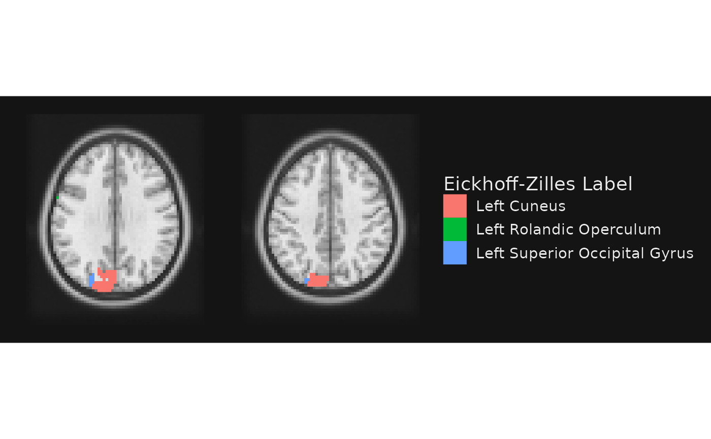
Notice how we went from four colors (one per number) in the previous plot to three labels here. Why did this happen? The labels for the four regions were not unique in the lookup atlas.
##   value                  CA_ML_18_MNI
## 1    12                   Left Cuneus
## 2    13                   Left Cuneus
## 3    14 Left Superior Occipital Gyrus
## 4    18       Left Rolandic Operculum
This highlights a useful point: there can be a one-to-many mapping between labels and unique integer values in the NIfTI image. Indeed, this is often an explicit goal. For example, what if we want to see the Yeo 7 networks assignments for the nodes on these two slices?
(Note that I’m removing the filter atlas < 20 here to
let all of the parcels on these slices get to play.)
gg_obj <- gg_base +
  geom_brain(definition = "atlas", name = "Yeo 7 Assignment",
             mapping = aes(fill = network))

plot(gg_obj)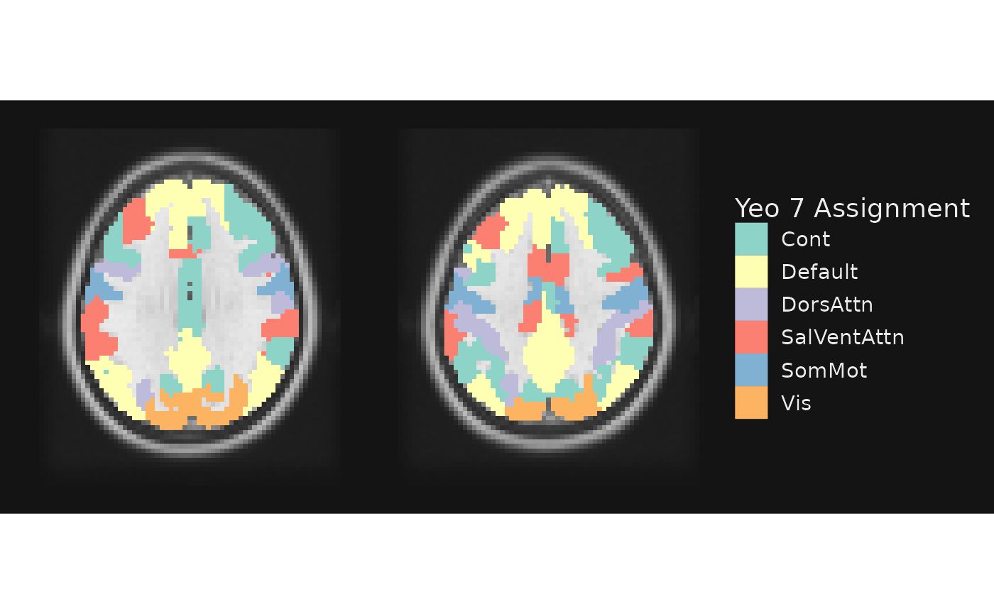
If we do not provide a color palette using the
fill_scale argument, it defaults to ColorBrewer’s
“Set3”, scale_fill_brewer(palette = "Set3").
What if we wanted to use the same coloration as in the original Yeo et al. 2011 paper? These colors are provided in the Yeo2011_7Networks_ColorLUT.txt file from Freesurfer.
yeo_colors <- read.table(system.file("extdata", "Yeo2011_7Networks_ColorLUT.txt", package = "ggbrain")) %>%
  setNames(c("index", "name", "r", "g", "b", "zero")) %>% slice(-1)

# Convert RGB to hex. Also, using a named set of colors with scale_fill_manual ensures accurate value -> color mapping
yeo7 <- as.character(glue::glue_data(yeo_colors, "{sprintf('#%.2x%.2x%.2x', r, g, b)}")) %>%
  setNames(c("Vis", "SomMot", "DorsAttn", "SalVentAttn", "Limbic", "Cont", "Default"))

gg_obj <- gg_base +
  geom_brain(definition = "atlas", name = "Yeo 7 Assignment",
             mapping = aes(fill = network), fill_scale = scale_fill_manual(values=yeo7))

plot(gg_obj)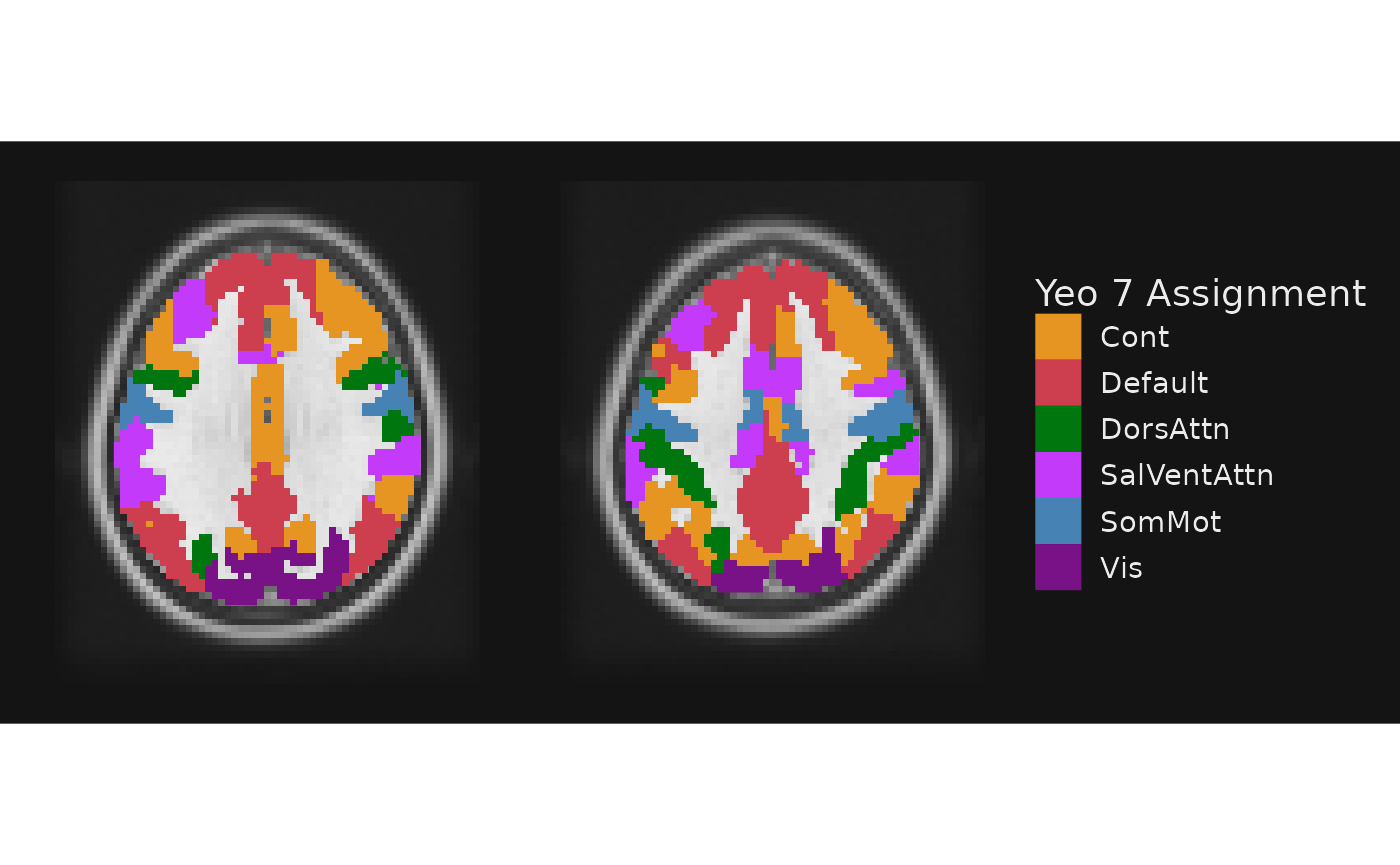
Combining filled areas with outlines
It may be useful to map some labels to the fill of an area and to
draw outlines around areas using another label. For example, if regions
are nested within networks, we might want to outline the networks with a
certain color while having separate colors for regions. This can be
achieved by adding a geom_outline layer for networks
alongside a geom_brain layer for regions.
gg_obj <- gg_base +
  geom_brain(definition = "DAN Region := atlas[atlas.network == 'DorsAttn']",
             mapping=aes(fill=CA_ML_18_MNI), show_legend = TRUE) +

  geom_outline(definition = "atlas", name = "Yeo 7 Assignment",
               mapping = aes(outline = network),
               outline_scale = scale_fill_manual(values=yeo7), show_legend = TRUE)

plot(gg_obj)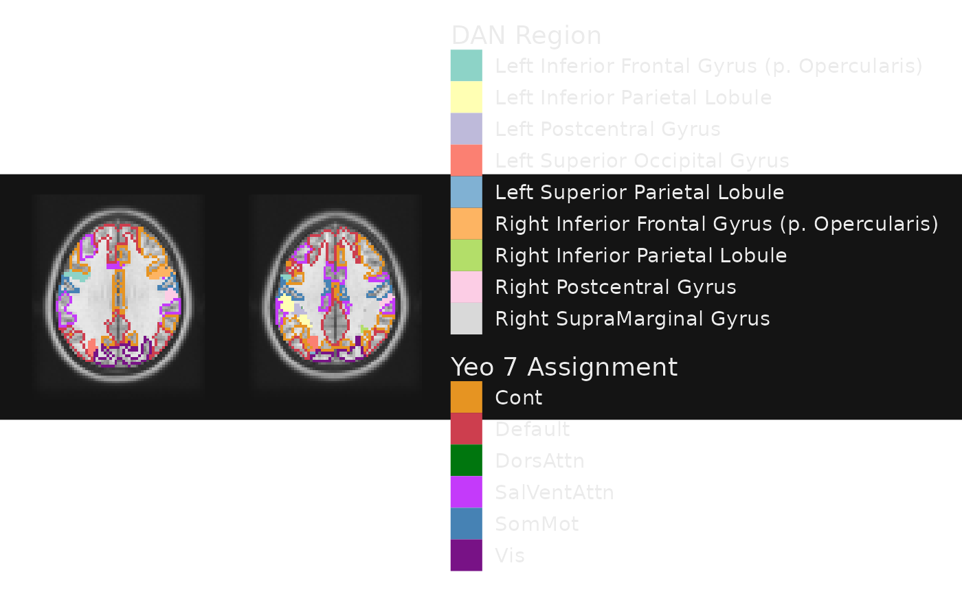
This admittedly a busy figure! But you get the idea of how to combine outlines and fills for these categorical images.
Combining quantitative layers with labels
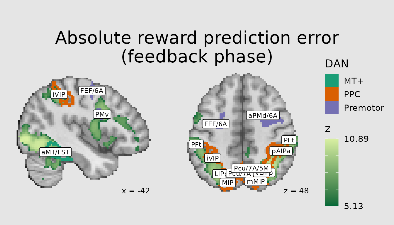
Another common use of atlases (and other categorical images) is to contextualize a pattern of activity from a voxelwise analysis in terms of its overlap with atlas parcels/regions. This can be achieved by combining a quantitative layer in ggbrain with a categorical one. Here, we plot the pattern of activity associated with absolute prediction errors from a study of reinforcement learning and overlay major regions of the Dorsal Attention Network, namely posterior parietal cortex (PPC), premotor (including frontal eye fields), and middle temporal visual area (MT+).
# first, divide relevant DAN parcels into groups
dan_labels <- schaefer200_atlas_labels %>%
  filter(network=="DorsAttn") %>%
  mutate(
    dan_group=case_when(
      value %in% c(31, 32, 135, 136) ~ "MT+",
      value %in% c(33:40, 137:144) ~ "PPC",
      value %in% c(41:43, 145:147) ~ "Premotor"
    )
  )

abspe_gg <- ggbrain(bg_color = "gray90", text_color = "black",
                    base_size = 16, title = "Absolute reward prediction error\n(feedback phase)") +
  images(c(underlay = underlay_file, overlay=abspe_overlay_3mm)) +
  images(c(atlas = schaefer200_atlas_file), labels=dan_labels) +
  slices(c("x = -42", "z = 49")) +
  geom_brain(definition = "underlay") +
  geom_brain(definition = "overlay", fill_scale = scale_fill_gradient("z", low="#006837", high="#d9f0a3"),
             breaks = range_breaks()) +
  geom_outline(definition = "atlas", mapping = aes(outline = dan_group),
               outline_scale = scale_fill_brewer("DAN", palette = "Dark2"), show_legend = TRUE, size=2) +
  annotate_coordinates(hjust = 1, color = "black", x = "right", y = "bottom")

render(abspe_gg) + plot_layout(nrow = 1, ncol = 2)
Adding annotations
In addition to plotting categorical images, we often wish to annotate
our plots with custom text in the margin or labels overlaid on certain
areas. ggbrain provides the annotate_slice function, which
allows you to add a custom annotation to one panel. This function
attaches to ggplot2::annotate such that any of its settings
apply to annotate_slice as well. Relative to typical
annotations in ggplot2, with ggbrain, we must also provide
x and y positions on the panel, as well the slice to which the
annotation should be added.
ann <- abspe_gg +
  annotate_slice(x=20, y=20, slice_index=1, geom="text", label="slice1", color="gray40", size=11, hjust=0) +
  annotate_slice(x=20, y=40, slice_index=2, geom="text", label="slice2", color="gray40", size=11, hjust=0)

plot(ann)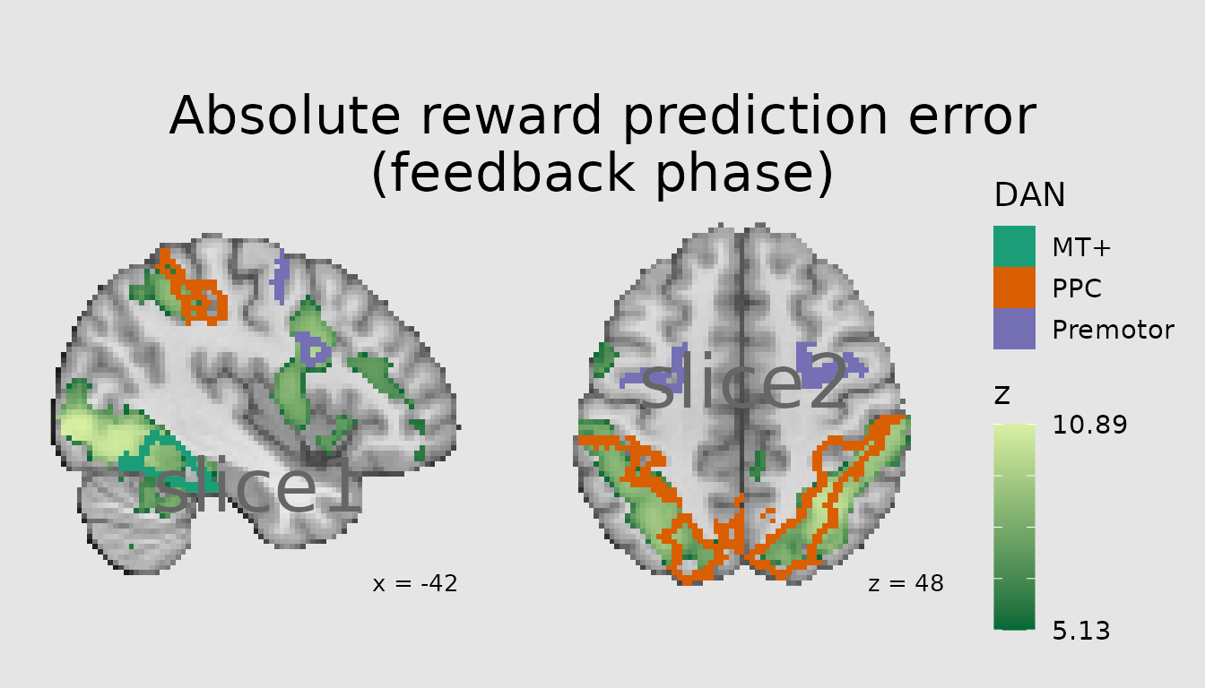
If numbers are provided for the x and y positions, these specify that the annotation should be placed at those coordinates in the pixel/voxel matrix. This may not be especially intuitive since we often don’t think about things in the matrix (aka “ijk” space) of the NIfTI. Here, our NIfTIs have dimensions: 97, 115, 97.
Alternatively, we can use the shorthand of “left” and “right” for x coordinates and “top” and “bottom” for y coordinates. The shorthand of “middle” also works in x and y.
ann <- abspe_gg +
  annotate_slice(x="left", y="top", slice_index=1, geom="text", label="slice1", color="gray40", size=11, hjust=0, vjust=1) +
  annotate_slice(x="right", y="bottom", slice_index=2, geom="text", label="slice2", color="gray40", size=11, hjust=1, vjust=0)

plot(ann)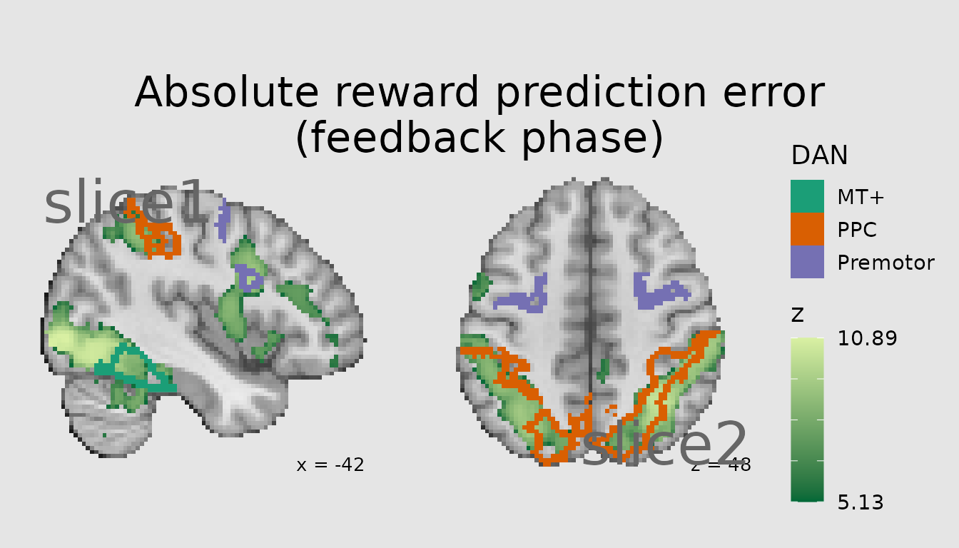
Finally, we can use quantiles/percentiles along each axis to position things in relative space.
ann <- abspe_gg +
  annotate_slice(x="q30", y="q60", slice_index=1, geom="text", label="slice1", color="gray40", size=11, hjust=0, vjust=1) +
  annotate_slice(x="q35", y="q70", slice_index=2, geom="text", label="slice2", color="gray40", size=11, hjust=0.5, vjust=0)

plot(ann)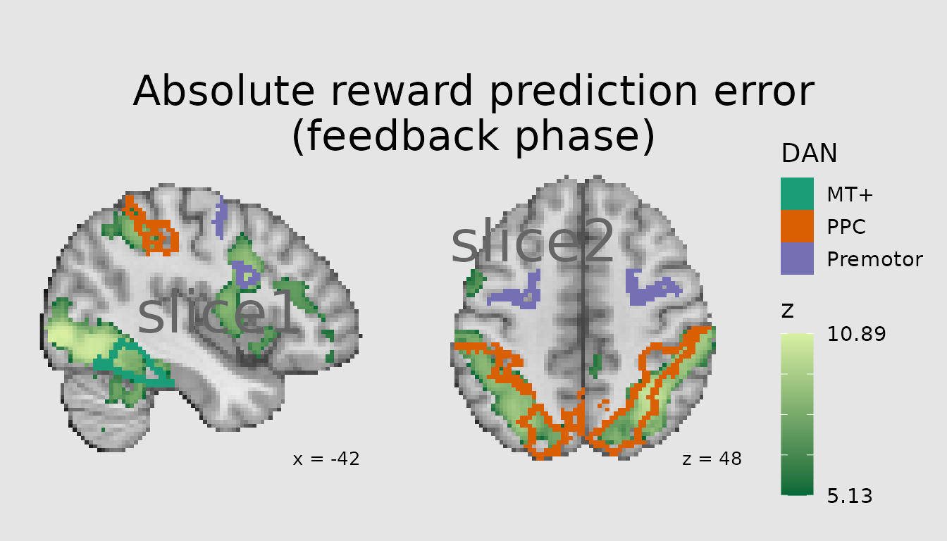
As with annotate in ggplot2, the
annotate_slice function can also be used to add other
geometric shapes such as rectangles or points. For example, we could
highlight the occipital region here.
ann <- abspe_gg +
  annotate_slice(xmin="q0", xmax="q38", ymin="q25", ymax="q59", slice_index=1, geom="rect",
                 color="blue", fill="transparent", linewidth=1.5)
plot(ann)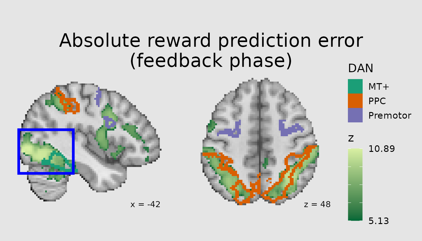
Adding labels systematically
Finally, we may wish to label points more systematically based on a
labeling data.frame, akin to how geom_text can
be used to label many points.
For example, we may want to add region labels to several regions on
the plot. To do this, ggbrain provides
geom_region_text, geom_region_text_repel,
geom_region_label, and
geom_region_label_repel.
The text versus label distinction matches
ggplot2, such that “label” annotations have a rectangle behind them
while “text” annotations do not.
The repel versions of these functions rely on ggrepel,
a useful package for pushing labels away from their specified
coordinates to avoid overplotting of labels and covering of relevant
data points.
Extending our plot above, perhaps we might like to label the Schaefer
parcellation regions comprising the three DAN areas of MT+, PPC, and
Premotor. These labels already exist in our
schaefer200_atlas_labels data.frame. Let’s use the
MNI_Glasser_HCP_v1.0 labels.
ann <- abspe_gg +
  geom_region_label(image="atlas", label_column="MNI_Glasser_HCP_v1.0", size=3, color="black")
#
#   geom_region_label_repel(image = "dan_clust", label_column = "value", min.segment.length = 0, size=3,
#                           color="black", force_pull=0, force=1.5, max.overlaps=Inf, box.padding = 0.5, label.padding=0.15, min_px = 20) +

plot(ann)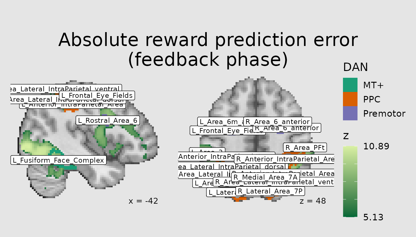
That’s clearly too busy! And those region labels are pretty long. We might instead use the automated labels alongside domain knowledge to create custom labels that are both potentially more accurate and also easier to read. Here, I’ve labeled a few of the regions in the DAN by looking at relevant literature and comparing it against anatomical labels. Although these labels are imperfect, they are more useful for visualization than the long labels.
## [1] "|MNI_Glasser_HCP_v1.0                 |custom_label |"
## [2] "|:------------------------------------|:------------|"
## [3] "|L_Area_PH                            |MT/MST       |"
## [4] "|L_Medial_Superior_Temporal_Area      |TPJ          |"
## [5] "|L_Area_V3A                           |iLIP         |"
## [6] "|L_Frontal_Eye_Fields                 |lFEF         |"
ann <- abspe_gg +
  geom_region_label(image="atlas", label_column="custom_label", size=3, color="black")
#
#   geom_region_label_repel(image = "dan_clust", label_column = "value", min.segment.length = 0, size=3,
#                           color="black", force_pull=0, force=1.5, max.overlaps=Inf, box.padding = 0.5, label.padding=0.15, min_px = 20) +

plot(ann)